Introduction

Proteins are nature's versatile nanomachines— they have evolved to perform virtually every important task in living systems. While nature has produced an incredible range of protein functions, these represent only a tiny fraction of what's possible in the protein universe. De novo protein design explores the full sequence space, guided by the physical principles that underlie protein folding. By exploring this vast pool of unexplored protein structures, it should be possible to design new functional proteins from the ground up to tackle current challenges in biomedicine and nanotechnology.

But rational protein design is tough. The search space is astronomical—even small proteins can have more possible sequences than atoms in the observable universe. Engineers must simultaneously optimize for structural stability and biological function, making the design process extremely complex. Traditional approaches combining physical modeling and directed evolution have been limited by their computational demands and the need for extensive experimental validation.

As with most other things, machine learning has been a transformative force in protein engineering, with models like AlphaFold2 (AF2) solving the decades-old problem of predicting how protein sequences fold into three-dimensional structures. However, structure prediction alone isn't enough for protein design - we need to generate novel proteins with specific properties. This requires models that can:

• Sample diverse but physically realistic protein structures
• Condition generation on desired properties (like binding to specific molecules)
• Account for protein flexibility and structural heterogeneity
• Generate structures that are different from natural proteins while maintaining stability

This led researchers to explore alternative approaches for protein generation. While early attempts using variational autoencoders (VAEs) struggled to capture the complex geometric constraints of protein structures, generative adversarial networks (GANs) faced challenges with training instability and mode collapse – producing limited diversity in their outputs. Diffusion models (DMs) offer several inherent advantages: they excel at modeling complex high-dimensional data, provide natural ways to incorporate geometric constraints, and allow flexible conditioning on desired properties. These characteristics have led to rapid adoption in structural biology, where DMs now achieve state-of-the-art results in de novo protein design, protein-ligand docking, etc. By combining insights from geometric deep learning with statistical physics principles, DMs can now match and surpass traditional techniques in computational structural biology.

Diffusion Models Overview

First, a quick primer on diffusion models as its crucial to understand how it is being used in protein design.

Diffusion models are a category of deep generative models that solve a fundamental challenge in machine learning: how to sample from complex, high-dimensional distributions in a computationally tractable way. Traditional approaches to sampling complex distributions, like Markov chain Monte Carlo (MCMC) simulations, can get stuck in local minima or struggle with high-dimensional spaces. Diffusion models sidestep these challenges by breaking down the generation process into a series of simpler, learnable steps. They start with pure random noise (which is easy to sample) and iteratively denoise it until a meaningful sample emerges. This progressive approach makes it possible to sample from distributions that would be intractable to model directly.

So rather than trying to learn the entire complex distribution at once, the model only needs to learn how to remove a small amount of noise at each step. This makes the learning problem more manageable and leads to high-quality results, even for very complex data distributions.

For readers interested in the mathematical details, I recommend Lilian Weng's blog post or Yang Song's blogpost. If you're already familiar with diffusion models, feel free to skip to the next section.

Technical Details of Diffusion Models

Now let's explore the different flavors of diffusion models used in protein engineering. Fair warning - there will be equations, but I'll try to break down what they actually mean in plain English. Feel free to skip to the 'Why This Matters for Proteins' sections if you want to cut to the chase. Again, this is only an overview. I'll be skipping over a lot of nuance and details here so we can get to the protein stuff. For more detailed explanations, the two blogposts I mentioned above would be a good place to start.

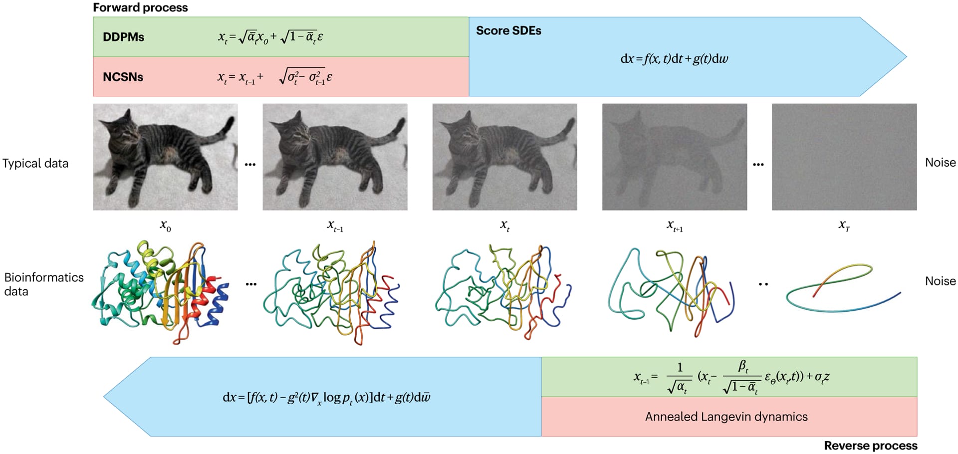
Denoising Diffusion Probabilistic Models (DDPMs)

DDPMs have two Markov chains: a forward diffusion process that progressively corrupts data with Gaussian noise, and a reverse process that learns to denoise it. Given a data distribution q(x₀), the forward process defines a sequence of latent variables through a fixed Markov chain with transition kernel q(xt​∣xt−1​):

$$q(x_t|x_{t-1}) = \mathcal{N}(x_t; \sqrt{1-\beta_t}x_{t-1}, \beta_t I)$$

where βₜ represents the variance schedule across diffusion steps, and I is the identity matrix. This forward process gradually corrupts the data by adding noise according to a predefined schedule until the data distribution approaches a standard Gaussian distribution. The reverse process aims to recover the data distribution by learning to denoise gradually. It is parameterized by a neural network that defines a sequence of conditional distributions:

$$p_\theta(x_{t-1} | x_t) = \mathcal{N}(x_{t-1}; \mu_\theta(x_t, t), \Sigma_\theta(x_t, t))$$

where μₜ and Σₜ represent the learned mean and variance parameters, respectively. By training a neural network to approximate μₜ(xₜ, t) (typically conditioned on xₜ and t), DDPMs learn to predict the original data point x₀ from a fully noisy input by gradually reversing the forward diffusion steps.

Training DDPMs involves minimizing the evidence lower bound (ELBO) on the negative log-likelihood of the data. This ELBO is derived from the variational objective and structured as a sum of denoising losses at each time step t, guiding the model to predict the noise added at each step accurately. A simplified version of the training loss function is:

$$L_\text{simple}(\theta) = \mathbb{E}_{x_0, \epsilon, t} \left[ \left\| \epsilon - \epsilon_\theta(x_t, t) \right\|^2 \right]$$

where ε represents the noise injected during the forward process, and εₜ is the model's prediction for that noise at each time step. This loss encourages the model to denoise accurately, so it can reconstruct x₀ by predicting and removing the noise.

Why This Matters for Proteins: The DDPM framework is particularly valuable for protein design because its step-by-step denoising process aligns well with how proteins fold—a series of small, coordinated changes rather than an abrupt transformation. The ability to control the noise schedule (βₜ) lets us carefully balance between exploring new structures and maintaining physical constraints. Also, the Gaussian noise assumption works surprisingly well for protein backbone coordinates, making DDPMs a natural choice for backbone generation tasks.

Noise-Conditioned Score Networks (NCSNs)

NCSNs, rather than directly modeling the data distribution p(x), estimate its score function ∇x log p(x)—the gradient of the log probability density with respect to the input. This approach, known as score matching, learns how to transform noisy samples back toward the true data distribution. The figure below illustrate this process: at each noise level σ, the arrows show the score function's gradient field, indicating how noisy samples (blue points) should move to better match the target distribution (orange regions). By learning these gradient fields at multiple noise levels (σ1, σ2, σ3), NCSNs can guide the sampling process without needing to compute complex normalizing constants typically required in likelihood-based models.

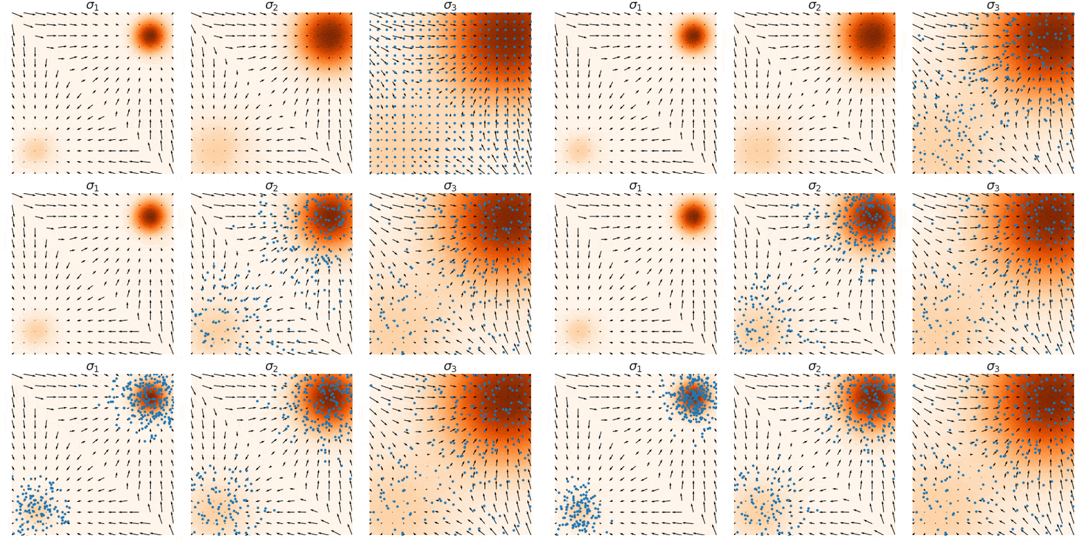
In practice, score matching on its own struggles with stability, especially in high-dimensional spaces, due to sparse data coverage across the distribution space. To address this, denoising score matching is often employed, where a small Gaussian noise is added to the data, creating a perturbed distribution q(x̃|x). By training on this corrupted data, the model learns a more robust approximation of the true score function, making it less sensitive to regions with sparse data coverage.

Further improvements are made by introducing sliced score matching, which leverages random projections to estimate scores more efficiently. This approach enables tractable, scalable training even with high-dimensional data, but it requires additional compute resources due to the use of multiple random projections.

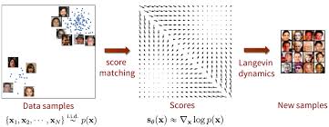
The sampling process in NCSNs utilizes Langevin dynamics, a Markov chain Monte Carlo (MCMC) method to generate new samples. Given an initial noise sample, Langevin dynamics iteratively refines it by following the learned score function direction while adding a small amount of random noise at each step. This ensures that the sampling process gradually converges to the target data distribution.

The key practical difference is that DDPMs often provide more stable training and sampling due to their fixed Markov structure, while NCSNs offer more flexibility in handling complex data geometries through their score-based formulation.

Why This Matters for Proteins: Score-based models are especially powerful for proteins because they can capture the complex energy landscape of protein structures. The score function essentially learns the gradient of this energy landscape, providing a natural way to guide sampling toward physically realistic conformations. This is particularly useful for tasks like molecular docking, where we need to find energetically favorable configurations. The multiple noise levels also help handle the multi-scale nature of protein structures—from local backbone geometry to global fold architecture.

Stochastic Differential Equations (SDEs)

When we consider diffusion models with continuous-time dynamics rather than discrete steps like in DDPMs or NCSNs, the perturbation and denoising processes can be described using stochastic differential equations (SDEs). This continuous formulation, known as score SDE, provides a mathematical framework where the forward process of adding noise follows an SDE. The solution to this process takes the form of an Itô SDE, which combines a drift term (controlling the mean transformation of the data) with a diffusion term (describing the noise addition).

In this framework, we learn a time-dependent score function st(x, t) = ∇x log pt(x), which captures how to gradually denoise the data at each point in the continuous process. This score function provides the direction that guides noisy samples back toward the clean data distribution.

The forward process is defined as:

$$dx=f(x,t)dt+g(t)dw$$

where:

• f(x, t) is the drift term, representing the deterministic part of the process, which dictates the overall direction or trend of the variable x.
• g(t) is the diffusion coefficient, controlling the intensity of the randomness.
• dw is the Wiener process (or Brownian motion), which represents a source of Gaussian noise with mean zero and variance dt.

To generate samples, we reverse this process with a reverse-time SDE. The reverse SDE requires knowledge of the score function (the gradient of the log density) at each point in time, and it is defined as:

$$dx= \left[f(x, t) - g(t)^2 \nabla_x \log p_t(x) \right] dt + g(t) dw$$

Here, ∇ₓ log pₜ(x) represents the score of the data distribution at time t, which is learned by a neural network during training. By solving this reverse SDE, we can transform Gaussian noise back into data samples, effectively generating new data points that follow the learned distribution.

The score function sₜ(x, t) is trained using a denoising score matching loss:

$$\mathcal{L}_{\text{DSM}} = \mathbb{E}_{t, x_t} \left[ \| s_\theta(x_t, t) - \nabla_{x_t} \log p_t(x_t) \|^2 \right]$$

Why This Matters for Proteins: The continuous nature of SDEs makes them ideal for modeling protein dynamics, which are inherently continuous processes. The ability to incorporate both deterministic (drift) and stochastic (diffusion) terms mirrors the physical reality of protein motion, where both directed forces and random thermal fluctuations play important roles. This framework also provides a natural way to incorporate physical constraints and prior knowledge about protein behavior through the drift term, while the diffusion term allows for exploration of conformational space.

Special Considerations for Diffusion Models in Proteins

Okay so, that was about diffusion models. But proteins have certain properties that need to be considered when applying diffusion models to protein design. When applying diffusion models to protein design, we need to handle two fundamental geometric properties of protein structures: invariance and non-Euclidean geometry.

Invariance

A protein's function depends on its shape and internal structure—how its atoms are arranged relative to each other—not on where it happens to be floating in space or which direction it's facing. Invariance refers to the property of a system or model to remain unchanged under certain transformations. It ensures that these of proteins properties are preserved even when the molecules undergo specific transformations, such as rotations and translations. Specifically, we want our model to be:

• Rotation Invariant: The model's predictions should not change if the entire molecular system is rotated in 3D space.
• Translation Invariant: The model's predictions should not change if the entire molecular system is translated (shifted) in 3D space.

To achieve this, we use special neural networks called E(3)-equivariant networks that preserve these 3D symmetries during the generation process. The "E(3)" refers to the mathematical group that describes all possible rotations and translations in 3D space. Models like ESM-IF1 use this approach because they need to model detailed atomic interactions.

Non-Euclidean Geometry

The second key consideration is that protein structures don't exist in simple flat (Euclidean) space. Instead, they're better described using internal coordinates like bond angles and torsion angles (φ, ψ, ω). These coordinates naturally exist in curved mathematical spaces called Riemannian manifolds.

This matters for two main reasons:

1. Dimensionality: Working with internal coordinates can significantly reduce the number of parameters needed to describe a protein structure
2. Physical Constraints: Using manifolds allows us to naturally enforce physical constraints like fixed bond lengths and angles

For example, RFdiffusion uses this approach for protein backbone generation since torsion angles naturally capture protein backbone flexibility with fewer parameters than atomic coordinates.

Applications

Ok whew!!! With all that said, let's finally dive into how diffusion models are actually being used in protein design. I'll focus on two major applications: protein backbone generation and molecular docking. Given how rapidly this field is evolving, this isn't an exhaustive list—but these examples showcase some of the most exciting use cases.

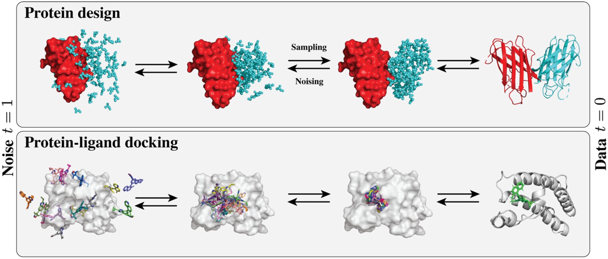
Protein Backbone Generation

Diffusion models lend themselves nicely to the design of proteins with specific functions or structural properties for protein engineering and drug discovery. Before diving into modern approaches, it's worth understanding how proteins can be represented for machine learning. At the simplest level, ignoring 3D geometric constraints, proteins can be represented in two main ways: as one-dimensional (1D) sequences of angles that define the backbone structure, or as two-dimensional (2D) contact and distance maps between residues. Early methods like ProteinSGM took the 2D approach, generating distance and angle matrices that were then processed through Rosetta to construct protein structures. While effective for both unconditional generation and inpainting tasks, this approach required computationally intensive post-processing steps.

Other approaches like FoldingDiff and DiffSDS explored the 1D angle-based representation, effectively treating protein backbone generation as a sequence modeling task. DiffSDS enhanced this by implementing a specialized encoder-decoder architecture where the encoder transforms invariant features into direction vectors, and the decoder reverses this transformation. While these approaches simplified the architecture, they struggled with error accumulation along the sequence and couldn't effectively handle multi-chain proteins.

A major paradigm shift came with the introduction of models that work directly with 3D coordinates, enabled by advances in geometric deep learning. These models needed to address a fundamental challenge: proteins can exist in any orientation or position in 3D space (SE(3) symmetry), but their fundamental structure remains the same. This led to SE(3)-equivariant neural networks, which ensure that rotating or translating the input protein produces correspondingly transformed outputs.

Early attempts like ProtDiff used Equivariant Graph Neural Networks (EGNNs) to generate protein backbone coordinates directly. However, these models were invariant to reflections, leading to physically unrealistic structures like left-handed alpha helices. A breakthrough came with Invariant Point Attention (IPA), originally developed for AlphaFold2, which represents proteins as a series of rigid body frames anchored at each residue. This preserves crucial information about angular relationships while maintaining SE(3)-equivariance, effectively capturing protein chirality. Models like Genie built upon this foundation, combining IPA with diffusion models to generate protein structures end-to-end.

The field has also made significant progress in conditional generation, particularly for tasks like motif scaffolding - where the goal is to design a protein structure (scaffold) that incorporates a specific functional element (motif). Early attempts like SMCDiff used sequential Monte Carlo sampling with an unconditional diffusion model to scaffold small motifs, though with limited success. RFdiffusion represented a major breakthrough by directly training on the motif scaffolding task, providing both sequence and structure of the motif while only diffusing the scaffold region. They also established the first comprehensive benchmark for motif scaffolding, demonstrating success across a range of functional motifs and achieving experimental validation.

Recent innovations have focused on improving efficiency and scalability. FrameDiff showed that comparable performance could be achieved without pre-trained structure predictors, while Chroma extended generation capabilities to proteins over 3,000 residues - far beyond previous limits. The field continues to move toward more controllable generation, with newer models handling various constraints like symmetry, shape, and specific functional sites, making protein design increasingly practical for real-world applications.

Molecular Docking

Think of molecular docking as figuring out how molecules fit together - like finding the right key (a small molecule) for a specific lock (a protein). The core task is to predict how a small molecule (called a ligand) will bind to a protein target - essentially finding both the location and orientation of the ligand that results in the most favorable interaction. Traditional approaches have relied on computationally expensive search algorithms that explore possible binding poses, combined with physics-based scoring functions to evaluate each possibility. While early deep learning attempts tried to directly predict binding poses through regression, they often fell short of traditional methods' performance. This changed with the introduction of diffusion models, which offered a more principled approach to generating and scoring potential binding configurations.

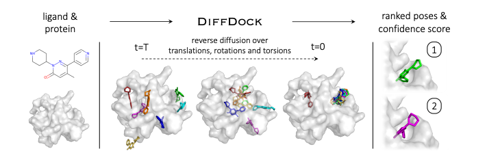
The application of diffusion models to molecular docking has spawned diverse strategies for predicting protein-ligand interactions, each addressing different aspects of the docking challenge. Initial approaches focused on the fundamental task of blind docking, where DiffDock pioneered the use of diffusion models to predict ligand positions without prior knowledge of binding sites. This method applied diffusion to ligand translation and rotation, using SE(3)-equivariant GNNs to sample and score multiple potential binding positions, significantly outperforming traditional search-based methods with a 38.2% success rate for top predictions.

Alternative strategies emerged for pocket-based docking, where binding site information is known in advance. DiffBP took a distinctive approach by eliminating the need for ligand structure input entirely - instead using a pre-generation network to determine the ligand's center of mass and atom count, followed by equivariant GNNs to generate complete ligand candidates. This method showed remarkable improvement in binding affinities, achieving 41.07% success compared to previous autoregressive methods that generated atoms sequentially.

A significant advancement came with models that addressed protein flexibility during docking. NeuralPLexer introduced an equivariant structure diffusion module that could accommodate changes in protein structure during ligand binding, working with a heterogeneous graph that incorporated both protein and ligand components. This approach achieved around 70% success rate for accurate ligand placement while maintaining low steric clash rates, demonstrating the value of incorporating protein flexibility in the diffusion process.

Some models focused on specific aspects of the docking problem. DiffSBDD specialized in generating new ligands for known protein pockets, offering both protein-conditioned generation and ligand inpainting capabilities. A particularly innovative approach emerged with the development of a deep generative energy-based diffusion model that could predict binding affinities without requiring labeled training data, using SE(3) denoising score matching to estimate ligand-protein interactions, performing comparably to traditional supervised methods.

Other Applications

Here I'll briefly touch on some other applications of diffusion models in protein design. The most exciting recent applications incorporate diffusion-based architecture that is capable of predicting the joint structure of complexes including proteins, nucleic acids, small molecules, ions and modified residues. This represents a significant shift from earlier approaches that treated different biomolecules as separate prediction tasks.

AlphaFold 3 exemplifies this trend by incorporating diffusion-based modeling to handle the joint prediction of diverse biomolecular structures. The model uses a diffusion process to gradually denoise and refine the entire complex simultaneously, allowing it to capture subtle interdependencies between different molecular types and their conformational changes. This unified approach helps predict how different components of a biological system interact and influence each other's structure. Similarly, Chai-1 extends this multimodal approach by using diffusion models to handle an even broader range of biomolecules, including post-translational modifications and non-standard amino acids. The diffusion process helps model the uncertainty in structure prediction while maintaining physical consistency across different molecular types.

In molecular dynamics, diffusion models are being explored as a way to generate new conformational trajectories and predict protein motion. Unlike traditional molecular dynamics simulations that rely on physics-based force fields, diffusion models can learn to generate physically plausible conformational changes directly from experimental data. This could potentially accelerate drug discovery by better predicting protein flexibility and dynamics.

Diffusion models have also shown promise in inverse folding - the task of designing sequences that will fold into a desired structure. By treating sequence generation as a denoising process guided by the target structure, these models can explore diverse sequence possibilities while maintaining compatibility with the desired fold.

Evaluation Challenges

The current evaluation landscape for protein diffusion models reveals significant gaps between what we can measure and what actually matters for real-world protein design. The dominant evaluation paradigm relies on what's called "self-consistency" - a pipeline where we take a generated protein backbone, use ProteinMPNN to design its sequence, and then feed that sequence into a structure predictor like AlphaFold2 or ESMFold to see if we get back our original structure. A protein is considered "designable" if this predicted structure closely matches the original (typically measured by an RMSD < 2.0 Å).

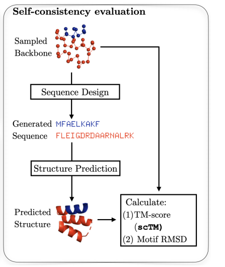
While self-consistency is useful and correlates with wet-lab success, it has major limitations. First, it's primarily focused on unconditional generation - basically asking "can we make stable proteins?" rather than "can we make proteins that do what we want?" This is particularly problematic because most real-world applications require conditional generation - designing proteins with specific binding sites, catalytic activities, or structural motifs. Unfortunately, we lack standardized benchmarks and metrics for these more complex tasks.

The metrics we do have also miss crucial aspects of protein design:

• They can't reliably evaluate protein-protein interactions or multimeric structures
• They don't tell us why certain designs fail
• They can be "gamed" by models that repeatedly generate the same safe structures rather than exploring diverse designs
• They don't directly measure the properties we actually care about, like binding affinity, catalytic activity, or manufacturability

To compensate for some of these issues, researchers typically report additional metrics like diversity (how different are the generated structures from each other?) and novelty (how different are they from known proteins in the PDB?). But these still don't capture functional success.

The situation is reminiscent of early language models being evaluated primarily on perplexity rather than actual task performance. Just as the field eventually developed more task-specific benchmarks like GLUE and SuperGLUE, protein diffusion models need standardized benchmarks that evaluate conditional generation, functional properties, and real-world applicability. Without these, it's difficult to meaningfully compare different approaches or guide the field toward solving practical protein design challenges.

Flow Matching

Flow matching represents an exciting evolution in generative modeling that could address some key challenges in protein design. Unlike traditional diffusion models that require many noising and denoising steps, flow matching directly learns a continuous-time vector field that transforms a simple noise distribution into complex protein structures in a single flow.

This approach is particularly promising for protein engineering for several reasons. First, the continuous nature of the flow could better capture the smooth conformational changes that proteins undergo - matching the physical reality of protein dynamics better than discrete diffusion steps. Second, flow matching models can potentially generate samples faster since they don't require multiple denoising steps.

Most intriguingly, flow matching provides a more direct way to incorporate physical constraints and domain knowledge. Rather than just learning to denoise, we can explicitly design the vector field to respect protein physics - like bond angles, atomic distances, and energetic considerations. This could lead to more reliable and physically realistic protein designs. In the protein space, ProteinFM demonstrated that flow matching could effectively generate protein backbone structures while maintaining physical constraints. FoldFlow extended this idea by incorporating structure prediction directly into the flow, enabling better control over the generated structures. FrameFlow, an adaptation of FrameDiff, used SE(3)-equivariant flows to generate protein backbones while preserving geometric constraints, demonstrating improved sampling efficiency and structure quality.

While flow matching for protein design is still in its early stages, it represents a natural evolution of diffusion-based approaches that could help overcome current limitations in generation speed and physical accuracy. As the field continues to develop better evaluation metrics and benchmarks, flow matching models may prove to be a powerful tool in the protein engineer's arsenal.

Conclusion

Diffusion models have emerged as a powerful new tool in the protein engineer's toolkit and the field is evolving rapidly, with flow matching models suggesting an exciting path toward faster, more physically grounded generation.

Our evaluation metrics still fall short of capturing what truly matters for real-world applications, and the gap between generating stable proteins and designing functional ones remains substantial. As the field matures, the development of better benchmarks, more sophisticated conditioning methods, and improved ways to incorporate physical constraints will be crucial.

Thanks for reading! While I've aimed for accuracy, I'm still learning and not an expert in this - so corrections and feedback are very welcome.